
2023-10-14-【学习】孟德尔随机化.md 17 KB
title: 【学习】孟德尔随机化 urlname: Mendelian-Randomization date: 2023-10-14 17:18:54 index_img: https://api.limour.top/randomImg?d=2023-10-14 17:18:54
tags: ['SNP', 'MR']
MR定义
孟德尔随机化是一种基于全基因组测序数据(GWAS数据),利用单核首酸多态性(SNPs)作为工具变量(IV),用于揭示因果关系的新型流行病学方法,相较于队列研究等观察性研究,暴露在出生前便已确定,较少受到反向因果及混杂因素的影响,因而能够有效减少偏倚。
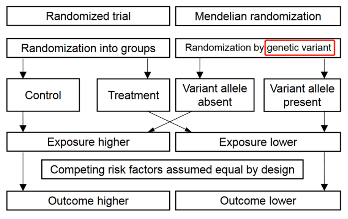 MR的核心是运用遗传学数据作为桥梁,来探索某一暴露和某一结局之间的因果关联。与RCT将参与者随机分配到试验组或对照组类似,MR研究基于影响危险因素的一个或多个等位基因,对参与基因进行"随机化"(自然的随机化),以确定这些遗传变异的携带者与非携带者相比,是否具有不同的疾病发生风险,因此,孟德尔随机化可以被认为类似于"自然的随机对照试验"。MR的相关术语
理论假设
- the variant is associated with the exposure
- the variant is not associated with the outcome via a confounding pathway
- the variant does not affect the outcome directly, only possibly indirectly via the exposure
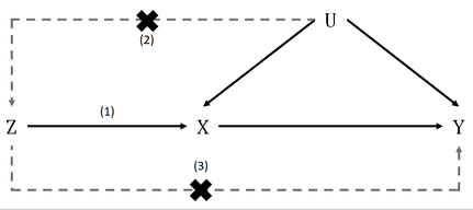
- 关联性假设:变异与暴露有关
- 独立性假设:变异与结果之间没有通过混杂途径相关
- 排他性假设:变异不直接影响结果,只可能通过暴露途径间接影响
- 关联性假设:p值,F统计量,R^2
- 排他性假设:与结局的相关性计算时,p值要大于0.05
MR-Egger回归相比线性回归可以弱化对排他性假设的要求
适用范围
不确定先有鸡还是先有蛋,比如,到底是抑郁导致肺癌还是肺癌导致了抑郁?
暴露因素难以测量,或者花费昂贵。例如,水溶性维生素等生物标志物的检测金标准可能成本太高,大样本无法承受,或者空腹血糖的测量需要隔夜空腹,可能不现实。
暴露与结局数据来自同一人群,且不存在或存在少量可接受范围内的样本重叠
配置环境
-
conda create -n MR -c conda-forge r-devtools -y
conda activate MR
conda install -c conda-forge r-irkernel -y
Rscript -e "IRkernel::installspec(name='MR', displayname='MR')"
# Rscript -e "usethis::edit_r_environ()" # 设置 GITHUB_PAT
# nano ~/.Renviron # MRCIEU 真是超喜欢GITHUB,要访问一万次 api.github.com
conda install -c conda-forge r-rmarkdown -y
conda install -c conda-forge r-meta -y
wget https://github.com/MRCIEU/TwoSampleMR/archive/refs/heads/master.zip -O TwoSampleMR.zip
Rscript -e "devtools::install_local('TwoSampleMR.zip')"
wget https://github.com/MRCIEU/MRInstruments/archive/refs/heads/master.zip -O MRInstruments.zip
Rscript -e "devtools::install_local('MRInstruments.zip')"
conda install -c conda-forge r-susier -y
conda install -c bioconda bioconductor-variantannotation -y
wget https://github.com/MRCIEU/gwasglue/archive/refs/heads/master.zip -O gwasglue.zip
Rscript -e "devtools::install_local('gwasglue.zip')"
# wget https://github.com/MRCIEU/genetics.binaRies/archive/refs/heads/master.zip -O genetics.binaRies.zip
# Rscript -e "devtools::install_local('genetics.binaRies.zip')"
conda install -c bioconda plink -y
# whereis plink # /opt/conda/envs/MR/bin/plink
Rscript -e 'install.packages("MendelianRandomization")'
数据来源
精神病学基因组:PGC
社会科学遗传学:SSGAC
大脑健康和疾病:CTG
MRCIEU汇总数据库:IEU
GWAS研究目录:NHGRI-EBI
-
一些参考数据
wget http://fileserve.mrcieu.ac.uk/ld/1kg.v3.tgz
tar -zxvf 1kg.v3.tgz
# mkdir EUR && mv EUR.* EUR
示例结局数据
-
# zcat ADHD2022_iPSYCH_deCODE_PGC.meta.gz | head
CHR SNP BP A1 A2 FRQ_A_38691 FRQ_U_186843 INFO OR SE P Direction Nca Nco
8 rs62513865 101592213 C T 0.925 0.937 0.981 0.99631 0.0175 0.8325 +---+++0-++-+ 38691 186843
8 rs79643588 106973048 G A 0.91 0.917 1 1.00411 0.0159 0.7967 ++--++-+-+-++ 38691 186843
8 rs17396518 108690829 T G 0.561 0.577 0.998 0.99611 0.0096 0.6876 --++-++??-+-- 37367 184388
8 rs983166 108681675 A C 0.57 0.586 0.996 0.99491 0.0096 0.5956 --++-++++-+-- 38691 186843
8 rs28842593 103044620 T C 0.839 0.836 0.982 0.98314 0.0135 0.2081 ----++0+??--+ 37504 184525
8 rs7014597 104152280 G C 0.824 0.824 0.997 0.99950 0.0122 0.9679 +-++-+++++--- 38691 186843
8 rs3134156 100479917 T C 0.841 0.833 0.997 0.98866 0.0128 0.3762 -+----+--++-- 38691 186843
8 rs6980591 103144592 A C 0.783 0.79 1 1.01106 0.0108 0.3075 ++-++---+++++ 38691 186843
8 rs72670434 108166508 A T 0.642 0.623 0.983 1.00672 0.0103 0.5171 +++-+++--+++- 38691 186843
CHR Chromosome (hg19) SNP Marker name BP Base pair location (hg19) A1 Reference allele for OR (may or may not be minor allele) A2 Alternative allele FRQ_A_38691 allele frequency of A1 in 38,691 ADHD cases FRQ_U_186843 allele frequency of A1 in 38,691 controls INFO Imputation information score (the reported imputation INFO score is a weighted average across the cohorts contributing to the meta-analysis for that variant) OR Odds ratio for the effect of the A1 allele SE Standard error of the log(OR) P P-value for association test in the meta-analysis Direction direction of effect in the included cohorts Nca number of cases with variant information Nco number of controls with variant information其中
SNP,Effect allele,Beta(OR),SE,P这五列是必须的。遇到没有提供EAF的数据,可以匹配千人基因组数据的EAF,get_eaf_from_1000G。示例暴露数据
wget -c https://gwas.mrcieu.ac.uk/files/ieu-a-2/ieu-a-2.vcf.gzVCF_dat = VariantAnnotation::readVcf('~/upload/GWAS/IEU/ieu-a-2.vcf.gz') exp_dat = gwasglue::gwasvcf_to_TwoSampleMR(vcf = VCF_dat) saveRDS(file = 'ieu-a-2.exp_dat', exp_dat) exp_dat = subset(exp_dat, pval.exposure < 5e-08) # 关联性假设 # 去除连锁不平衡 # exp_dat = TwoSampleMR::clump_data(dat = exp_dat, clump_kb = 10000, clump_r2 = 0.001) # MRCIEU太喜欢用cloud api了 fix_ld_clump_local = function (dat, tempfile, clump_kb, clump_r2, clump_p, bfile, plink_bin) { shell <- ifelse(Sys.info()["sysname"] == "Windows", "cmd", "sh") write.table(data.frame(SNP = dat[["rsid"]], P = dat[["pval"]]), file = tempfile, row.names = F, col.names = T, quote = F) fun2 <- paste0(shQuote(plink_bin, type = shell), " --bfile ", shQuote(bfile, type = shell), " --clump ", shQuote(tempfile, type = shell), " --clump-p1 ", clump_p, " --clump-r2 ", clump_r2, " --clump-kb ", clump_kb, " --out ", shQuote(tempfile, type = shell)) print(fun2) system(fun2) res <- read.table(paste(tempfile, ".clumped", sep = ""), header = T) unlink(paste(tempfile, "*", sep = "")) y <- subset(dat, !dat[["rsid"]] %in% res[["SNP"]]) if (nrow(y) > 0) { message("Removing ", length(y[["rsid"]]), " of ", nrow(dat), " variants due to LD with other variants or absence from LD reference panel") } return(subset(dat, dat[["rsid"]] %in% res[["SNP"]])) } fuck = fix_ld_clump_local( dat = dplyr::tibble(rsid=exp_dat$SNP, pval=exp_dat$pval.exposure), tempfile = file.path(getwd(),'tmp.ld_clump.exp_dat'), clump_kb = 10000, clump_r2 = 0.001, clump_p = 1, # pop = "EUR", # Super-population. Options are "EUR", "SAS", "EAS", "AFR", "AMR" plink_bin = '/opt/conda/envs/MR/bin/plink', # 千万别用什么 genetics.binaRies::get_plink_binary(),他们自己编译的文件有问题 bfile = "/home/jovyan/upload/GWAS/ld/EUR" # 前缀,不是文件夹也不是文件 ) exp_dat_clumped = exp_dat[exp_dat$SNP %in% fuck$rsid,] saveRDS(file = 'ieu-a-2.exp_gwas', exp_dat_clumped)获取暴露数据
自己的数据
df_gwas <- data.frame(
SNP = c("rs1", "rs2"),
beta = c(1, 2),
se = c(1, 2),
effect_allele = c("A", "T")
)
head(df_gwas)
exp_dat <- TwoSampleMR::format_data(df_gwas, type = "exposure")
gwas_catalog
df_gwas <-
subset(MRInstruments::gwas_catalog,
     grepl("Speliotes", Author) &
       Phenotype == "Body mass index")
head(df_gwas)
exp_dat <- TwoSampleMR::format_data(df_gwas)
metab_qtls
df_gwas <-
subset(MRInstruments::metab_qtls,
    phenotype == "Ala"
)
head(df_gwas)
exp_dat <- TwoSampleMR::format_metab_qtls(df_gwas)
proteomic_qtls
df_gwas <-
subset(MRInstruments::proteomic_qtls,
    analyte == "ApoH"
)
head(df_gwas)
exp_dat <- TwoSampleMR::format_proteomic_qtls(df_gwas)
某个基因
df_gwas <-
subset(MRInstruments::gtex_eqtl,
    gene_name == "IRAK1BP1" & tissue == "Adipose Subcutaneous"
)
head(df_gwas)
exp_dat <- TwoSampleMR::format_gtex_eqtl(df_gwas)
某个性状的某个甲基化位点相关QTL
df_gwas <-
subset(MRInstruments::aries_mqtl,
    cpg == "cg25212131" & age == "Birth"
)
head(df_gwas)
exp_dat <- TwoSampleMR::format_aries_mqtl(df_gwas)
IEU的ID
exp_gwas <- TwoSampleMR::extract_instruments(outcomes = 'ieu-a-2')
head(exp_gwas)
saveRDS(file = 'ieu-a-2.exp_gwas', exp_gwas) # 和自己从VCF开始经过clump得到的差不多
UK_Biobank
hyperten_tophits <- ieugwasr::tophits(id="ukb-b-12493", clump=0)
hyperten_gwas <- dplyr::rename(hyperten_tophits, c(
"SNP"="rsid",
"effect_allele.exposure"="ea",
"other_allele.exposure"="nea",
"beta.exposure"="beta",
"se.exposure"="se",
"eaf.exposure"="eaf",
"pval.exposure"="p",
"N"="n"))
fuck = fix_ld_clump_local(
dat = dplyr::tibble(rsid=hyperten_gwas$SNP, pval=hyperten_gwas$pval.exposure),
tempfile = file.path(getwd(),'tmp.ld_clump.exp_dat'),
clump_kb = 10000, clump_r2 = 0.001, clump_p = 1,
# pop = "EUR", # Super-population. Options are "EUR", "SAS", "EAS", "AFR", "AMR"
plink_bin = '/opt/conda/envs/MR/bin/plink', # 千万别用什么 genetics.binaRies::get_plink_binary(),他们自己编译的文件有问题
bfile = "/home/jovyan/upload/GWAS/ld/EUR" # 前缀,不是文件夹也不是文件
)
exp_dat_clumped = hyperten_gwas[hyperten_gwas$SNP %in% fuck$rsid,]
MR_calc_r2_F(
beta = exp_dat_clumped$beta.exposure, # Vector of Log odds ratio. beta = log(OR)
eaf = exp_dat_clumped$eaf.exposure, # Vector of allele frequencies.
N = exp_dat_clumped$N, # Array of sample sizes
se = exp_dat_clumped$se.exposure # Vector of SE.
) # 取 F>10 的
计算统计效力
# 分类变量
tmp_r2 =TwoSampleMR::get_r_from_lor(
lor = exp_dat_clumped$beta.exposure, # Vector of Log odds ratio. beta = log(OR)
af = exp_dat_clumped$eaf.exposure, # Vector of allele frequencies.
ncase = exp_dat_clumped$ncase.exposure, # Vector of Number of cases.
ncontrol = exp_dat_clumped$ncontrol.exposure, # Vector of Number of controls.
prevalence = 1, # Vector of Disease prevalence in the population.
)
# 连续变量
tmp_r2 =TwoSampleMR::get_r_from_pn(
p = exp_dat_clumped$pval.exposure, # Array of pvals
n = exp_dat_clumped$samplesize.exposure # Array of sample sizes
)
MR_calc_r2_F = function(beta, eaf, N, se){ # https://doi.org/10.1038/s41467-020-14389-8 # https://doi.org/10.1371/journal.pone.0120758 r2 = (2 * (beta^2) * eaf * (1 - eaf)) / (2 * (beta^2) * eaf * (1 - eaf) + 2 * N * eaf * (1 - eaf) * se^2) F = r2 * (N - 2) / (1 - r2) print(mean(F)) return(dplyr::tibble(r2=r2, F=F)) } MR_calc_r2_F( beta = exp_dat_clumped$beta.exposure, # Vector of Log odds ratio. beta = log(OR) eaf = exp_dat_clumped$eaf.exposure, # Vector of allele frequencies. N = exp_dat_clumped$samplesize.exposure, # Array of sample sizes se = exp_dat_clumped$se.exposure # Vector of SE. ) # 取 F>10 的获取结局数据
IEU
out_gwas = TwoSampleMR::extract_outcome_data(snps = exp_gwas$SNP, outcomes = 'ieu-a-7')UK_Biobank
anxiety_hyperten_liberal <- TwoSampleMR::extract_outcome_data(snps = exp_dat_clumped$SNP, outcomes = "ukb-b-11311")PGC的示例
df_gwas = read.table(gzfile('~/upload/GWAS/PGC/ADHD2022_iPSYCH_deCODE_PGC.meta.gz'), header = T)
head(df_gwas)
df_gwas = df_gwas[df_gwas$SNP %in% exp_gwas$SNP,]
out_gwas = data.frame(
SNP = df_gwas$SNP,
chr = as.character(df_gwas$CHR),
pos = df_gwas$BP,
beta.outcome = log(df_gwas$OR),
se.outcome = df_gwas$SE,
samplesize.outcome = df_gwas$Nca + df_gwas$Nco,
pval.outcome = df_gwas$P,
eaf.outcome = with(df_gwas, (FRQ_A_38691*Nca+FRQ_U_186843*Nco)/(Nca+Nco)),
effect_allele.outcome = df_gwas$A1,
other_allele.outcome = df_gwas$A2,
outcome = 'ADHD',
id.outcome = 'ADHD2022_iPSYCH_deCODE_PGC'
)
out_gwas = subset(out_gwas, pval.outcome > 5e-08) # 排他性假设
附加 代理SNP
一部分暴露的SNPs在结局中找不到,可以找和这部分SNPs连锁不平衡的SNPs来代替。相关网站:snipa
Harmonization
- 将Exposure-SNP及Outcome-SNP等位基因方向协同
- 根据EAF大小,剔除不能判断方向的回文SNP
剔除incompatible SNP
dat <- TwoSampleMR::harmonise_data(
exposure_dat = exp_gwas,
outcome_dat = out_gwas
)
附加 一键报告
TwoSampleMR::mr_report(dat, output_type = "md")MR分析
回归分析
TwoSampleMR::mr_method_list() # 查看mr支持的MR分析方法
mr_regression = TwoSampleMR::mr(dat, method_list = c('mr_ivw', 'mr_egger_regression', 'mr_weighted_median'))
mr_regression_or = TwoSampleMR::generate_odds_ratios(mr_res = mr_regression) # 分类变量
{pdf(file = 'MR.BMIvsADHD.plot.pdf', width = 6, height = 6); # 导出 PDF 开始
print(TwoSampleMR::mr_scatter_plot(mr_results = mr_regression, dat = dat)); # 返回的是一个ggplot2对象
dev.off()} # 导出 PDF 结束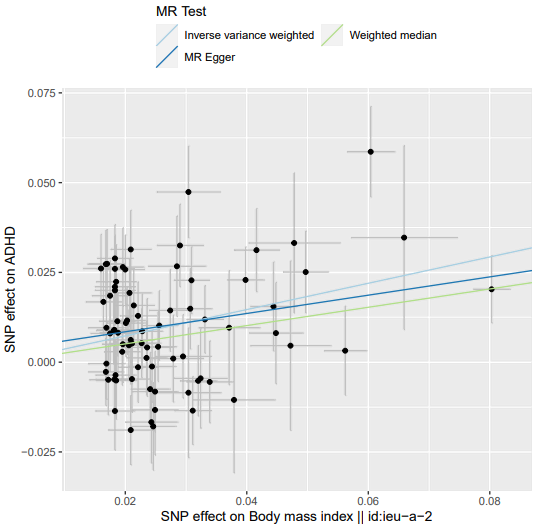
异质性检测
有异质性用随机效应模型
ivw,无异质性用固定效应模型(也可以用随机效应模型,两者结果一致)异质性可能带来多效性,如果没有多效性,则可以说异质性没有带来多效性
TwoSampleMR::mr_heterogeneity(dat) # ivw的 Q_pval < 0.05 则说明有异质性
heterogeneity_presso = TwoSampleMR::run_mr_presso(dat, NbDistribution = 3000) # NbDistribution越高分辨率越高,找不到离群的SNP时需要提高
heterogeneity_presso[[1]]$`MR-PRESSO results`$`Global Test`$Pvalue # < 0.05 说明有异质性
heterogeneity_presso[[1]]$`MR-PRESSO results`$`Distortion Test`$`Outliers Indices` # 显示离群的SNP,将其剔除后重新分析
水平多效性
P < 0.05 说明不满足独立性假设,建议放弃继续做这个课题
P < 0.05 拒绝了截距为0的假设,说明SNP效应为0时依然有影响(截距存在),有其他因素在起作用
TwoSampleMR::mr_pleiotropy_test(dat)敏感性分析
Leave-one-out analysis
所有结果都不应该存在跨过0的情况,否则说明结果不稳定,不再能说明因果关系
mr_loo <- TwoSampleMR::mr_leaveoneout(dat)
{pdf(file = 'MR.BMIvsADHD.leaveoneout.plot.pdf', width = 6, height = 6); # 导出 PDF 开始
print(TwoSampleMR::mr_leaveoneout_plot(leaveoneout_results = mr_loo)); # 返回的是一个ggplot2对象
dev.off()} # 导出 PDF 结束
单SNP分析
对每个暴露-结果组合进行多次分析,每次使用不同的单 SNP 进行分析
mr_res_single <- TwoSampleMR::mr_singlesnp(dat)
TwoSampleMR::mr_funnel_plot(mr_res_single)
TwoSampleMR::mr_forest_plot(mr_res_single)
方向性检测
TwoSampleMR::directionality_test(dat) # TRUE表示确实是暴露导致了结果附加 稳健回归
dat2 <- TwoSampleMR::dat_to_MRInput(dat)
mr_ivw_robust <- MendelianRandomization::mr_ivw(dat2[[1]], model= "default", # “random”指的就是随机效应模型,“fixed”指的是固定效应模型
                                         robust = TRUE, penalized = TRUE,correl = FALSE, # 参数penalized代表下调异常值的权重
                                         weights ="simple", psi = 0,distribution = "normal",alpha = 0.05)
附加 绘制森林图
附加 计算Power
- Calculating statistical power in Mendelian randomization studies
- Power calculations for Mendelian Randomization
- Sample size: 结局总的样本量,不是暴露的样本量
- K: 结局中病例的比例,case/(case+control)
- OR: IVW的OR值,exp(beta)
- R2: MR_calc_r2_F 计算得到的所有R2的sum